Gridded EWH
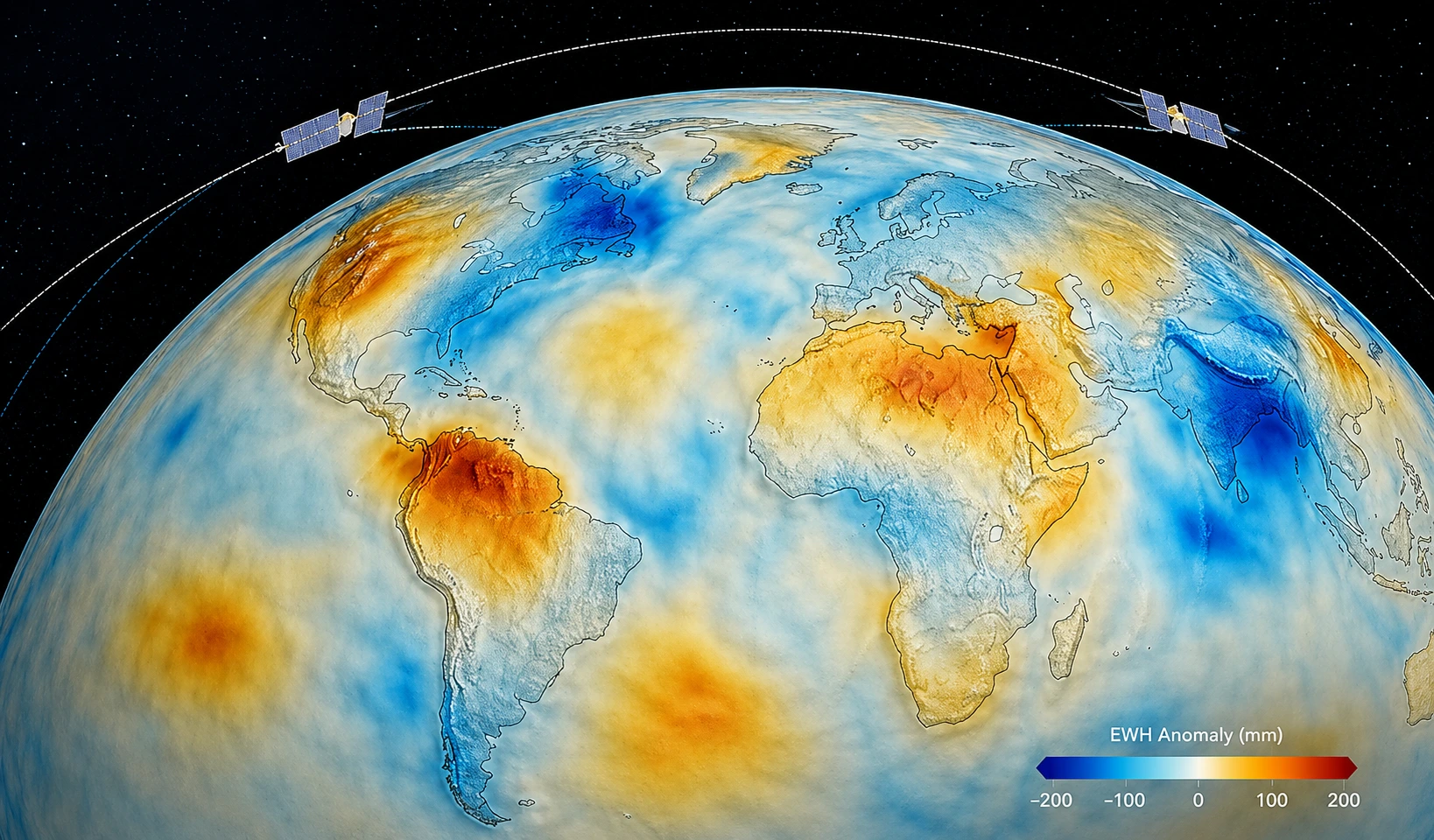
Monthly equivalent-water-height anomalies on controlled grids with product metadata and diagnostics.
Read preview noteSatellite Gravity Field
From GSM spherical harmonics to gridded EWH products
Technical notes and reproducible workflow records for transforming GRACE and GRACE-FO Level-2 spherical harmonic solutions into physically consistent equivalent water height products.
00
Start from a topic, then move between workflow notes, method records, data products, and software releases.
Acquire, preprocess, filter, synthesize, and validate Level-2 products.
MethodsFiltering notesCompare Gaussian, decorrelation, DDK, HSAF, and leakage correction routes.
DataProducts and referencesTrack GSM coefficients, EWH grids, Mascon references, masks, and diagnostics.
ArticlesReproducible recordsRead project notes with assumptions, checks, and processing contracts.
01
Click any processing node to inspect the scientific contract behind the step.
Input should be treated as a Level-2 gravity-field solution, usually monthly GSM spherical harmonic coefficients. The product name, processing center, release, maximum degree/order, time stamp, missing month flag, and reference frame must remain explicit.
Preprocessing converts monthly coefficients into a consistent anomaly field. Typical operations include degree-1 geocenter replacement, C20/C30 replacement using SLR, GIA correction, optional destriping preconditions, and subtraction of a stated mean field.
Filtering reduces correlated north-south striping and random high-degree noise while preserving physically interpretable mass signals. Gaussian, Fan, PnMm decorrelation, DDK, and HSAF should be routed as separate products rather than overwritten arrays.
Spherical harmonic synthesis converts corrected coefficients into equivalent water height. The Love-number correction, Earth radius, water density, grid resolution, land/ocean mask, and units must be consistent across products.
Validation should combine visual quality control with quantitative diagnostics. Basin-mean time series, annual amplitude, trend, leakage-corrected regional products, Mascon comparison, hydrology models, and altimetry are separate evidence layers.
02
Keep data products explicit, versioned, and auditable.
Monthly equivalent-water-height anomalies on controlled grids with product metadata and diagnostics.
Read preview note
Independent products for checking spatial patterns, basin averages, and long-term behavior.
Read workflow note03
A compact record of each filter family and its routing contract.
Baseline filter families for reproducible comparison and controlled product tags.
Read article04
Latest notes from the processing log.
Access versioned installers, release notes, and software usage information from the download page.
Good processing is transparent, testable, and reproducible.
Workflow first, results follow.